Research_In_Computing

Research In Computing Practicals

M. Sc (Information Technology) PSIT1P1 Research In Computing

Index

Sr.No.	Name	README
Prac1A(Python) Prac1A(Excel)	1 A. Write a program for obtaining descriptive statistics of data.	prac1a(Python) prac1a(Excel)
Prac1B-1(From_CSV)(Python) Prac1B-1(Excel)	1 B. Import data from different data sources (from csv to R/Python/Excel)	prac1b-1(Python) prac1b-1(excel)
Prac1B-2(From_Excel)(Python) Prac1B-2(From_Excel)(Excel)	1 B. Import data from different data sources (from Excel to R/Python/Excel)	prac1b-2(Python) prac1b-2(excel)
Prac2A(Google Form)	2 A. Design a survey form for a given case study, collect the primary data and analyse it	prac2a
Prac2B(Excel)	2 B. Perform analysis of given secondary data.	prac2b(Excel)
Prac3A(Python)	3 A. Perform testing of hypothesis using one sample t-test.	prac3a
Prac3B(Python) Prac3B(Excel)	3 B. Write a program for t-test comparing two means for independent samples.	prac3b prac3b(excel)
Prac3C(Python)	3 C. Perform testing of hypothesis using paired t-test.	prac3c(Python)
Prac4A(Excel)	4 A. Perform testing of hypothesis using chi-squared goodness-of-fit test.	prac4a(Excel)
Prac4B(Python) Prac4B(Excel)	B. Perform testing of hypothesis using chi-squared Test of Independence.	prac4b prac4b(excel)
Prac5A(Python)	5 A. Perform testing of hypothesis using Z-test.	prac5a(Python)
Prac5B(Python)	5 B. Two-Sample Z test	prac5b(Python)
Prac6A(Excel)	6 A. Perform testing of hypothesis using one-way ANOVA	prac6a(excel)
Prac6B(Excel)	6 B. Perform testing of hypothesis using two-way ANOVA.	prac6b(excel)
Prac6C(Python)	6 C. Perform testing of hypothesis using multivariate ANOVA (MANOVA)	prac6c(Python)
Prac7A(Excel)	7 A. Perform the Random sampling for the given data and analyse it.	prac7a(excel)
Prac7B(Python)	7 B. Perform the Stratified sampling for the given data and analyse it	prac7b(Python)
Prac8A(Python) Prac8B(Python) Prac8C(Python)	Compute different types of correlation. 8A. Positive Correlation: 8B. Negative Correlation: 8C. No/Weak Correlation:	prac8a(Python) prac8b(Python) prac8c(Python)
Prac9A(Python)	9A. Write a program to Perform linear regression for prediction.	prac9a(Python)
Prac9B(Python) Prac9B(Excel)	9B. Perform polynomial regression for prediction.	prac9b(Python) prac9b(Excel)

---

Prac1A

• Practical 1A: Write a python program on descriptive statistics analysis.

#Practical 1A: Write a python program on descriptive statistics analysis.
################################################################
import pandas as pd
#Create a Dictionary of series
d = {'Age':pd.Series([25,26,25,23,30,29,23,34,40,30,51,46]),
'Rating':pd.Series([4.23,3.24,3.98,2.56,3.20,4.6,3.8,3.78,2.98,4.80,4.10,3.65])}
#Create a DataFrame
df = pd.DataFrame(d)
print(df)
print('############ Sum ########## ')
print (df.sum())
print('############ Mean ########## ')
print (df.mean())
print('############ Standard Deviation ########## ')
print (df.std())

OUTPUT

🔝

---

Prac1A(Excel)

• Practical 1A(Excel). Write a program for obtaining descriptive statistics of data.

Steps(Excel) & OUTPUT

1. Open Excel file.

2. Go to File -> Options -> Add-ins -> Click on Analysis Toolpack -> click on Go

   

3. Tick mark Analysis toolpack -> click on OK -> The Data Analysis option will be added in Data tab

   

4. Now click on Data analysis -> Descriptive Statistiscs -> click on OK

   

5. Click on input range -> select Age column in input column -> and select any blank column in output range -> Tick Mark on Summery statistics, confidence level for mean(95%), kth Largest(1), kth smallest(1). -> click on Ok

   

• Output:

  

🔝

---

Prac1B-1

• Import data from different data sources (from Excel, csv, mysql, sql server, oracle to R/Python/Excel)
• From csv

#1B-1.	Import data from different data sources (from Excel, csv, mysql, sql server, oracle to R/Python/Excel)
#From csv
import sqlite3 as sq
import pandas as pd
Base='C:/VKHCG'
sDatabaseName=Base + '/01-Vermeulen/00-RawData/SQLite/vermeulen.db'
conn = sq.connect(sDatabaseName)
sFileName='C:/VKHCG/01-Vermeulen/01-Retrieve/01-EDS/02-Python/Retrieve_IP_DATA.csv'
print('Loading :',sFileName)
IP_DATA_ALL_FIX=pd.read_csv(sFileName,header=0,low_memory=False)
IP_DATA_ALL_FIX.index.names = ['RowIDCSV']
sTable='IP_DATA_ALL'
print('Storing :',sDatabaseName,' Table:',sTable)
IP_DATA_ALL_FIX.to_sql(sTable, conn, if_exists="replace")
print('Loading :',sDatabaseName,' Table:',sTable)
TestData=pd.read_sql_query("select * from IP_DATA_ALL;", conn)
print('## Data Values')
print(TestData)
print('################')
print('## Data Profile')
print('################')
print('Rows :',TestData.shape[0])
print('Columns :',TestData.shape[1])
print('### Done!! ############################################')

OUTPUT

🔝

---

Prac1B-1(Excel)

• To Import data from csv file.

Steps(Excel) & OUTPUT

1. In Data tab, Click on Get Data.

2. Select From file -> Select From Text/CSV

   

3. Select the csv file and Click on Import

4. Preview window will open -> click on Load

   

5. The File will be Imported and will be shown.

   

🔝

---

Prac1B-2

• Import data from different data sources (from Excel, csv, mysql, sql server, oracle to R/Python/Excel)
• From Excel

#1B-2.	Import data from different data sources (from Excel, csv, mysql, sql server, oracle to R/Python/Excel)
#From Excel
import os
import pandas as pd
Base='F:/tmp/practical-data-science/VKHCG'
sFileDir=Base + '/01-Vermeulen/01-Retrieve/01-EDS/02-Python'

CurrencyRawData = pd.read_excel('F:/tmp/practical-data-science/VKHCG/01-Vermeulen/00-RawData/Country_Currency.xlsx')
sColumns = ['Country or territory', 'Currency', 'ISO-4217']
CurrencyData = CurrencyRawData[sColumns]
CurrencyData.rename(columns={'Country or territory': 'Country', 'ISO-4217': 'CurrencyCode'}, inplace=True)
CurrencyData.dropna(subset=['Currency'],inplace=True)
CurrencyData['Country'] = CurrencyData['Country'].map(lambda x: x.strip())
CurrencyData['Currency'] = CurrencyData['Currency'].map(lambda x: x.strip())
CurrencyData['CurrencyCode'] = CurrencyData['CurrencyCode'].map(lambda x: x.strip())
print(CurrencyData)

print('~~~~~~ Data from Excel Sheet Retrived Successfully ~~~~~~~ ')

OUTPUT

🔝

---

Prac1B-2(Excel)

• To Import data from Excel file.

Steps(Excel) & OUTPUT

1. In Data tab, Click on Get Data

2. Select From file -> Select From Excel Workbook.

   

3. Select the Excel worksheet to import -> click on OK

4. Navigator Window will open -> Select the sheets you want to import -> Click on Load

   

5. Data will be imported from the selected file and will be displayed

   

🔝

---

Prac2A(Google Form)

• Design a survey form for a given case study, collect the primary data and analyse it.

Steps(Google Form) & OUTPUT

🔝

---

Prac2B(Excel)

• Perform analysis of given secondary data.

Steps(Excel) & OUTPUT

1. Open World_population 2010 excel file.

2. Find the sum of Male and Female Column.

   

3. Create and find total of Male and Female coloumn
   (=B4+C4)

   

4. Find Sum of all Total column values.

   

5. Find Percentage of Male
   (= -1*100*male column value/ sum of all total values)
(=-1*100*B4/$D$22).

   

6. Find Percentage of Male
   (= 100*Female column value/ sum of all total values)
(100*C4/$D$22).

7. Find sum of both male% and female%

8. Select Male% and Female% -> insert -> clustered Bar

   

9. Put the tip of your mouse arrow on the Y-axis (vertical axis) so it says “Category Axis”, right click and chose Format Axis

   

10. Choose Axis options tab and set the major and minor tick mark type to None, Axis labels to Low, and click OK

11. Click on any of the bars in your pyramid, click right and select “format data series”. Set the Overlap to 100 and Gap Width to 0. Click OK.

• OUTPUT

  

🔝

---

Prac3A

• Perform testing of hypothesis using one sample t-test

#3A.Perform testing of hypothesis using one sample t-test.
#Google colab
from scipy.stats import ttest_1samp
import numpy as np

ages = np.genfromtxt("/content/ages.csv")
print(ages)
ages_mean = np.mean(ages)
print(ages_mean)
tset, pval = ttest_1samp(ages, 30)
print("p-values - ", pval)
if pval < 0.05:  # alpha value is 0.05
    print(" we are rejecting null hypothesis")
else:
    print("we are accepting null hypothesis")

OUTPUT

🔝

---

Prac3B

• Perform testing of hypothesis using two sample t-test

#3B-Perform testing of hypothesis using two sample t-test.
#Google colab
import numpy as np
from scipy import stats
from numpy.random import randn

N = 20
a = 5 * randn(100) + 50
b = 5 * randn(100) + 51
var_a = a.var(ddof=1)
var_b = b.var(ddof=1)
s = np.sqrt((var_a + var_b) / 2)
t = (a.mean() - b.mean()) / (s * np.sqrt(2 / N))
df = 2 * N - 2
# p-value after comparison with the t
p = 1 - stats.t.cdf(t, df=df)
print("t = " + str(t))
print("p = " + str(2 * p))
if t > p:
    print("Mean of two distribution are differnt and significant")
else:
    print("Mean of two distribution are same and not significant")

OUTPUT

🔝

---

Prac3B(Excel)

• Write a program for t-test comparing two means for independent samples.

Steps(Excel) & OUTPUT

1. Open Excel file.

2. Find the average(mean) of both Experimental and comparison columns.

   

3. Find the Standard deviation of both Experimental and comparison columns.

   

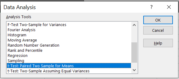
4. Go to Data analysis -> Select t-test: Paired Two Sample for Means -> OK.

   

5. For Variable 1 range(Experimental)= A1 to A21
   For Variable 2 range(Comparison)= B1 to B21
   For Output Range= D5 to F17

   

6. Write 2 Hypothesis
   H0 - Difference in gain score is not likely the result of experiment.
   H1 - Difference in gain score is likely the result of experimental treatment and not the result of change variation.

7. To calculate the T-Test square value go to cell E20 and type
   =(A22-B22)/SQRT((A23*A23)/COUNT(A2:A21)+(B23*B23)/COUNT(A2:A21))
   Formula =(Mean A-Mean B)/SQRT((STDEV A*STDEV B)/COUNT(of A) + (STDEV*STDEV)/COUNT(of A))

   

8. Now go to cell E21 and type
   =IF(E20<E12,"H0 is Accepted", "H0 is Rejected and H1 is Accepted")

• OUTPUT

🔝

---

Prac3C

• Perform testing of hypothesis using paired t-test.

#3C-Perform testing of hypothesis using paired t-test.
#Google colab
from scipy import stats
import matplotlib.pyplot as plt
import pandas as pd
df = pd.read_csv("blood_pressure.csv")
print(df[['bp_before','bp_after']].describe())
#First let’s check for any significant outliers in
#each of the variables.
df[['bp_before', 'bp_after']].plot(kind='box')
# This saves the plot as a png file
plt.savefig('boxplot_outliers.png')
#################**#############################
# make a histogram to differences between the two scores.
df['bp_difference'] = df['bp_before'] - df['bp_after']
df['bp_difference'].plot(kind='hist', title= 'Blood Pressure Difference Histogram')
#Again, this saves the plot as a png file
#################**#############################
plt.savefig('blood pressure difference histogram.png')
stats.probplot(df['bp_difference'], plot= plt)
plt.title('Blood pressure Difference Q-Q Plot')
plt.savefig('blood pressure difference qq plot.png')
stats.shapiro(df['bp_difference'])
stats.ttest_rel(df['bp_before'], df['bp_after'])

OUTPUT

🔝

---

Prac4A(Excel)

• Perform testing of hypothesis using chi-squared goodness-of-fit test.

Steps(Excel) & OUTPUT

1. Find total of both columns.

   

2. Enter the Formula.

   

3. Find the sum of all

   

4. At cell D7 type
   =CHIINV(0.05,2)

5. At cell D8 type
   =IF(D5>D7, "H0 Accepted","H0 Rejected").

• OUTPUT

  

🔝

---

Prac4B(Excel)

• Perform testing of hypothesis using chi-squared test of independence.

Steps(Excel) & OUTPUT

1. Find the total for all columns and rows.

   

2. To calculate the expected value Ei
   Go to Cell N9 and type =N8/2
   Go to Cell O9 and type =O8/2
   Go to Cell P9 and type =P8/2
   Go to Cell Q9 and type =Q8/2
   Go to Cell R9 and type =R8/2

   

3. Go to cell T6 and type
   =SUM((N6-$N$9)^2/$N$9,(O6-$O$9)^2/$O$9,(P6-$P$9)^2/$P$9,(Q6-Q$9)^2/$Q$9, (R6-$R$9)^2/$R$9)
   Go to cell T7 and type =SUM((N7-$N$9)^2/$N$9,(O7-$O$9)^2/$O$9,(P7-$P$9)^2/$P$9,(Q7-Q$9)^2/$Q$9, (R7-$R$9)^2/$R$9)

4. To get the table value go to cell T11 and type
   =CHIINV(0.05,4)

5. Go to cell O13 and type
   =IF(T8>=T11," H0 is Accepted", "H0 is Rejected")

• OUTPUT

  

🔝

---

Prac4B

• Perform testing of hypothesis using chi-squared

# Google colab
import numpy as np
import pandas as pd
import scipy.stats as stats

np.random.seed(10)
stud_grade = np.random.choice(
    a=["O", "A", "B", "C", "D"], p=[0.20, 0.20, 0.20, 0.20, 0.20], size=100
)
stud_gen = np.random.choice(a=["Male", "Female"], p=[0.5, 0.5], size=100)
mscpart1 = pd.DataFrame({"Grades": stud_grade, "Gender": stud_gen})
print(mscpart1)
stud_tab = pd.crosstab(mscpart1.Grades, mscpart1.Gender, margins=True)
stud_tab.columns = ["Male", "Female", "row_totals"]
stud_tab.index = ["O", "A", "B", "C", "D", "col_totals"]
observed = stud_tab.iloc[0:5, 0:2]
print(observed)
expected = np.outer(stud_tab["row_totals"][0:5], stud_tab.loc["col_totals"][0:2]) / 100
print(expected)
chi_squared_stat = (((observed - expected) ** 2) / expected).sum().sum()
print("Calculated : ", chi_squared_stat)
crit = stats.chi2.ppf(q=0.95, df=4)
print("Table Value : ", crit)
if chi_squared_stat >= crit:
    print("H0 is Accepted ")
else:
    print("H0 is Rejected ")

OUTPUT

🔝

---

Prac5A

• Perform testing of hypothesis using Z-test.

# Google colab
#A.	Perform testing of hypothesis using Z-test.
from statsmodels.stats import weightstats as stests
import pandas as pd
from scipy import stats

df = pd.read_csv("blood_pressure.csv")
df[["bp_before", "bp_after"]].describe()
print(df)
ztest, pval = stests.ztest(df["bp_before"], x2=None, value=156)
print(float(pval))
if pval < 0.05:
    print("reject null hypothesis")
else:
    print("accept null hypothesis")

OUTPUT

🔝

---

Prac5B

• Two-Sample Z test

# Google colab
# B.	Two-Sample Z test
import pandas as pd
from statsmodels.stats import weightstats as stests

df = pd.read_csv("blood_pressure.csv")
df[["bp_before", "bp_after"]].describe()
print(df)
ztest, pval = stests.ztest(
    df["bp_before"], x2=df["bp_after"], value=0, alternative="two-sided"
)
print(float(pval))
if pval < 0.05:
    print("reject null hypothesis")
else:
    print("accept null hypothesis")

OUTPUT

🔝

---

Prac6A(Excel)

• Perform testing of hypothesis using one-way ANOVA

Steps(Excel) & OUTPUT

1. Open scores.csv file

2. Go to Data analysis -> Anova single factor -> ok

   

3. Select input range as all values from [Average Score (SAT Math), Average Score (SAT Reading), Average Score (SAT Writing)] columns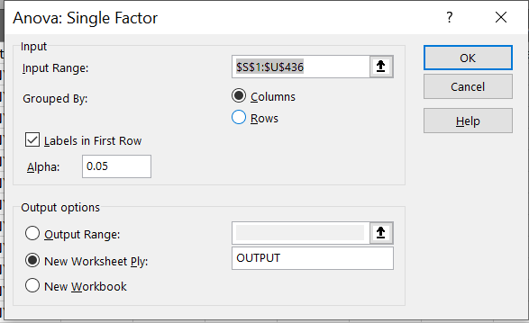

   

• OUTPUT

  

🔝

---

Prac6B(Excel)

• Perform testing of hypothesis using two-way ANOVA.

Steps(Excel) & OUTPUT

1. Open ToothGrowth.csv file

2. Go to Data analysis -> Anova two factor with replication -> ok.

   

3. Select all cell in input range ,
   Rows per sample=30
   Alpha=0.05

   

• OUTPUT

  

🔝

---

Prac6C

• Perform testing of hypothesis using multivariate ANOVA (MANOVA)

# Google colab
import pandas as pd
from statsmodels.multivariate.manova import MANOVA
df = pd.read_csv('Iris.csv', index_col=0)
df.columns = df.columns.str.replace(".", "_")
df.head()
print('~~~~~~~~ Data Set ~~~~~~~~')
print(df)
maov = MANOVA.from_formula('SepalLengthCm + SepalWidthCm + \
PetalLengthCm + PetalWidthCm ~ Species', data=df)
print('~~~~~~~~ MANOVA Test Result ~~~~~~~~')
print(maov.mv_test())

OUTPUT

🔝

---

Prac7A(Excel)

• Perform the Random sampling for the given data and analyse it.

Steps(Excel) & OUTPUT

1. Open existing excel sheet with population data.
   Sample Sheet looks as given below:
   Set Cell O1 = Male and Cell O2 = Female

2. To generate a random sample for male students from given population go to Cell O1 and type
   =INDEX(E$2:E$62,RANK(B2,B$2:B$62))
   Drag the formula to the desired no of cell to select random sample.

3. Now, to generate a random sample for female students go to cell P1 and type
   =INDEX(K$2:K$40,RANK(H2,H$2:H$40))
   Drag the formula to the desired no of cell to select random sample.

   

• OUTPUT

  

🔝

---

Prac7B

• Perform the Stratified sampling for the given data and analyse it.
• We are to carry out a hypothetical housing quality survey across Lagos state,Nigeria. And we looking at a total of 5000 houses (hypothetically). We don’t just go to one local government and select 5000 houses, rather we ensure that the 5000 houses are a representative of the whole 20 local government areas Lagos state is comprised of. This is called stratified sampling. The population is divided into homogenous strata and the right number of instances is sampled from each stratum to guarantee that the test-set (which in this case is the 5000 houses) is a representative of the overall population. If we used random sampling, there would be a significant chance of having bias in the survey results.

# Google colab
import pandas as pd
import numpy as np
import matplotlib
import matplotlib.pyplot as plt
plt.rcParams['axes.labelsize'] = 14
plt.rcParams['xtick.labelsize'] = 12
plt.rcParams['ytick.labelsize'] = 12
import seaborn as sns
color = sns.color_palette()
sns.set_style('darkgrid')
import sklearn
from sklearn.model_selection import train_test_split
housing =pd.read_csv('housing.csv')
print(housing.head())
print(housing.info())
#creating a heatmap of the attributes in the dataset

correlation_matrix = housing.corr()
plt.subplots(figsize=(8,6))
sns.heatmap(correlation_matrix, center=0, annot=True, linewidths=.3)
corr =housing.corr()
print(corr['median_house_value'].sort_values(ascending=False))
sns.distplot(housing.median_income)
plt.show()

OUTPUT

🔝

---

Prac8A

• 8.Write a program for computing different correlation
• A. Positive Correlation:

# Google colab
#8.Write a program for computing different correlation
#A.	Positive Correlation:
import numpy as np
import matplotlib.pyplot as plt
np.random.seed(1)
# 1000 random integers between 0 and 50
x = np.random.randint(0, 50, 1000)
# Positive Correlation with some noise
y = x + np.random.normal(0, 10, 1000)
np.corrcoef(x, y)
matplotlib.style.use('ggplot')
plt.scatter(x, y)
plt.show()

OUTPUT

🔝

---

Prac8B

• B. Negative Correlation:

# Google colab
#8.Write a program for computing different correlation
#B.	Negative Correlation: 
import numpy as np
import matplotlib.pyplot as plt
np.random.seed(1)
# 1000 random integers between 0 and 50
x = np.random.randint(0, 50, 1000)
# Negative Correlation with some noise
y = 100 - x + np.random.normal(0, 5, 1000)
np.corrcoef(x, y)
plt.scatter(x, y)
plt.show()
print("Practical 8-B")

OUTPUT

🔝

---

Prac8C

• 8C. No/Weak Correlation:

# Google colab
#8.Write a program for computing different correlation
#C.	No/Weak Correlation:
import numpy as np
import matplotlib.pyplot as plt
np.random.seed(1)
x = np.random.randint(0, 50, 1000)
y = np.random.randint(0, 50, 1000)
np.corrcoef(x, y)
plt.scatter(x, y)
plt.show()
print("Practical 8-C")

OUTPUT

🔝

---

Prac9A

• 9A. Write a program to Perform linear regression for prediction.

# PRAC 9A #Jupyter
#A.	Write a program to Perform linear regression for prediction.
import quandl, math
import numpy as np
import pandas as pd
from sklearn.model_selection import train_test_split
from sklearn import svm
from sklearn.linear_model import LinearRegression
import matplotlib.pyplot as plt
from matplotlib import style
import datetime

style.use("ggplot")
df = quandl.get("WIKI/GOOGL")
df = df[["Adj. Open", "Adj. High", "Adj. Low", "Adj. Close", "Adj. Volume"]]
df["HL_PCT"] = (df["Adj. High"] - df["Adj. Low"]) / df["Adj. Close"] * 100.0
df["PCT_change"] = (df["Adj. Close"] - df["Adj. Open"]) / df["Adj. Open"] * 100.0
df = df[["Adj. Close", "HL_PCT", "PCT_change", "Adj. Volume"]]
forecast_col = "Adj. Close"
df.fillna(value=-99999, inplace=True)
forecast_out = int(math.ceil(0.01 * len(df)))
df["label"] = df[forecast_col].shift(-forecast_out)
X = np.array(df.drop(["label"], 1))
X = preprocessing.scale(X)
X_lately = X[-forecast_out:]
X = X[:-forecast_out]
df.dropna(inplace=True)
y = np.array(df["label"])
X_train, X_test, y_train, y_test = sklearn.model_selection.train_test_split(
    X, y, test_size=0.2
)
clf = LinearRegression(n_jobs=-1)
clf.fit(X_train, y_train)
confidence = clf.score(X_test, y_test)
forecast_set = clf.predict(X_lately)
df["Forecast"] = np.nan
last_date = df.iloc[-1].name
last_unix = last_date.timestamp()
one_day = 86400
next_unix = last_unix + one_day
for i in forecast_set:
    next_date = datetime.datetime.fromtimestamp(next_unix)
    next_unix += 86400
df.loc[next_date] = [np.nan for _ in range(len(df.columns) - 1)] + [i]
df["Adj. Close"].plot()
df["Forecast"].plot()
plt.legend(loc=4)
plt.xlabel("Date")
plt.ylabel("Price")
plt.show()

print("Practical 9-A")

OUTPUT

🔝

---

Prac9B

• 9B Perform polynomial regression for prediction.

# PRAC 9B
# B.	Perform polynomial regression for prediction.
# Google colab
import numpy as np
import matplotlib.pyplot as plt


def estimate_coef(x, y):
    # number of observations/points
    n = np.size(x)
    # mean of x and y vector
    m_x, m_y = np.mean(x), np.mean(y)
    # calculating cross-deviation and deviation about x
    SS_xy = np.sum(y * x) - n * m_y * m_x
    SS_xx = np.sum(x * x) - n * m_x * m_x
    # calculating regression coefficients
    b_1 = SS_xy / SS_xx
    b_0 = m_y - b_1 * m_x
    return (b_0, b_1)


def plot_regression_line(x, y, b):
    # plotting the actual points as scatter plot
    plt.scatter(x, y, color="m", marker="o", s=30)
    # predicted response vector
    y_pred = b[0] + b[1] * x
    # plotting the regression line
    plt.plot(x, y_pred, color="g")
    # putting labels
    plt.xlabel("x")
    plt.ylabel("y")
    # function to show plot
    plt.show()


def main():
    # observations
    x = np.array([0, 1, 2, 3, 4, 5, 6, 7, 8, 9])
    y = np.array([1, 3, 2, 5, 7, 8, 8, 9, 10, 12])
    # estimating coefficients
    b = estimate_coef(x, y)
    print("Estimated coefficients:\nb_0 = {} b_1 = {}".format(b[0], b[1]))
    # plotting regression line
    plot_regression_line(x, y, b)


if __name__ == "__main__":
    main()
print("Practical 9-B")

OUTPUT

🔝

---

Prac9B(Excel)

• Perform polynomial regression for prediction.

Steps(Excel) & OUTPUT

1. Insert the data as follows

   

2. Go to Data -> Data Analysis -> Regression

   

3. Enter the input range and output range

   

4. Click on OK

   

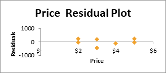
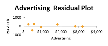
5. Select the PREDICTED QUANTITY SOLD and RESIDUALS column and paste on above table

   

• OUTPUT:

  

• Result: R square equals 0.962, which is a very good fit. 6% of the variation in Qunatity Sold is explained by the independent variables Price and Advertising. The closer to 1, the better the regression line (read on) fits the data.
  Significance F is 0.001464128 which is less than 0.05 (good fit).

🔝

---

Go To Top